Related Resources: math

Explicit Second Order Calculus Differential Equation Simulator Tool

Explicit Second Order Calculus Differential Equation Simulator Tool

Open (new Browser Window):
Explicit second order differential equation Simulator Tool

The simulation calculates solutions of ordinary explicit second order differential equations.

y´ ´= d ²y/ dx = f( y, y´, x)

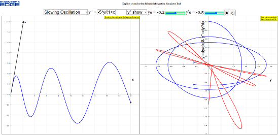
using the Runge−Kutta algorithm. In the left coordinate system the abscissa represents x, the ordinate y.

 

When opening the file you see a fat red point at x = 0, representing the initial value y₀ at its abscissa x₀ . You can change the initial value with the slider, more exactly and unlimited by typing a value into the number field. Two additional number fields are used to define x₀ and x_{max .} Default values are: y₀ = 1; x₀ = 0; x_max = 3. You can also draw the red point to create new initial conditions of y.

 

With a second slider you can define the initial value for the first derivative. It corresponds to the gradient at the initial ordinate, which is symbolized by an arrow.

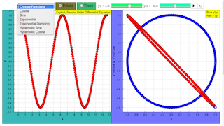
In the ComboBox you can chose between a number of predefined types of functions. Their formula is shown in field y´´ = ... There you can edit formulas or input any arbitrary first order explicit differential equation.

Activating start for the default equation, the differential equation of the exponential function y´´= y is evaluated. Calculation stops as x = x_max . At first you see a set of calculated points. You can choose the option trace to see an interpolated curve.

Stop stops the calculation; back leaves already calculated points and sets back to the initial conditions. Changing these now creates an additional curve at start. This way you can create sets of solutions for different initial conditions (the trace option would create jumps, which are avoided in the points option). Clear resets and clears traces, but leaves parameters unchanged. Reset leads back to default values..

After back you can change the x-resolution of calculation by slider step, and look how different resolutions influence the result.

The smaller window shows the phase space projections

y ´ = y ´( y )

y´´  = y´´ ( y )

The thick points are the last ones calculated.

The phase space diagrams very distinctively demonstrate the different character of solutions:  convergence, divergence, periodic oscillation, oscillating divergence, oscillating convergence. It is independent of the initial condition.

---

Numerical integration of differential equations with simulator

Using this differential equation simulator it is very easy to solve differential equations. Several algorithms for different methods are programmed and can be chosen at page Evolution with a mouse click. The steps of the variable x are automatically calculated, when the difference dx has been defined.

Differential equations of order n are separated into n coupled first order differential equations by substitution, and are calculated accordingly. For a 2nd order equation this leads to

y´´ = f( y, y´, x) ➔ y´ = dy/dx and y´´ = f( y, y´, x)

In this simulation with a ComboBox the formula is:

y´´ = (formula in field y´´, evaluated for x, y and y´)

This simulator presents the following methods : 

---

In all experiments study the phase space diagrams too!

E 1: Run cosine and try the points and the trace option.

What do the phase space projections mean?

Try different step widths.

E 2: Go back, and chose new initial conditions. Start creates the solution, which is different from the first one.
Try points an trace option.
E 3:  Create a set of solutions with identical initial value for y and different ones for y´. What is the result of different y´ for the sine function?
E 4:  Create a set of solutions with identical y₀ and different x₀. Why do you see curves that are shifted parallel?
E 5:  Create a set of curves with different initial values for y and y´, including negative ones. Interpret the results by analyzing the differential equation..
E 6: First choose Exponential, then Exponential Damping. Observe the phase space diagrams. What is the difference? Change initial values and compare again.
E 7:  Choose hyperbolic sine with default initial values y = 1 y´= 1.
Now choose hyperbolic cosine with default initial values y = 1 y´= 0.

Analyze the phase space diagrams.

Remarks:  For the normal exponential the gradient at x = 0 is equal to the initial value of y and cannot be zero for a meaningful exponential. Gradient zero for finite y is characteristic for the hyperbolic cosine (e ^x + e^{- x})/2, gradients > 0 with initial y = 0 for the hyperbolic sine (e ^x- e^{- x})/2. Imagine both functions mirrored at the zero-ordinate for completeness.

 

E 8: Choose slowing oscillation and study how the dependence on x influences the periods. Edit the formula such that frequency increases and slowing decreases.
E 9: Choose increasing oscillation and edit formulas correspondingly. Compare the effect of proportional and of reciprocal dependencies on x. Try nonlinear dependencies.
E 10: Choose damped oscillation. Check if periods are constant (when clicking at a point its coordinates are shown in the lower left corner).
E 11:  Choose increasing oscillation and compare the results to those of damped oscillation. Superimpose both curves and check if periods are equal.
E 12: Draw conclusions as to which consequences different terms in the differential equation have. With that in mind, construct differential equations that will show specific characteristics.

Related:

​Mechanics and Machine Design, Equations and Calculators

Credits:

Created by Dieter Roess in March 2009